Wednesday, May 28th, 2014
Hash functions are an essential mathematical tool that are used to translate data of arbitrary size into a fixed sized output. There are many different kinds of these functions, each with their own characteristics and purpose.
For example, cryptographic hash functions can be used to map sensitive information into hash values with high dispersion, causing even the slightest changes in the source information to produce wildly different hash results. Because of this, two cryptographic hashes can (usually) only be compared to determine if they came from the exact same source. We cannot however measure the similarity of two cryptographic hashes to ascertain the similarity of the sources.
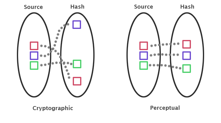
Perceptual hashes are another category of hashing functions that map source data into hashes while maintaining correlation. These types of functions allow us to make meaningful comparisons between hashes in order to indirectly measure the similarity between the source data.
Insight: Perceptual Image Hashing
Insight is a simple perceptual image hashing system that can compare two images and measure their similarity. For the remainder of this post we will walk through the inner workings of Insight, and examine a common use case for perceptual hashing: reverse image searches.
Let's suppose that we have the following image, and we want to search the web for similar images. We're interested in anything that is structurally similar, and not necessarily identical.
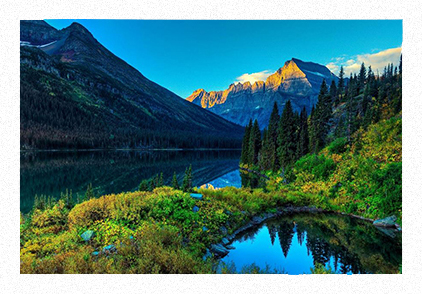
Figure 1: Our query image
Our web crawler quickly presents us with a candidate image that we wish to compare against our query image. At this point we invoke our perceptual image hashing system to generate hashes of both images. To accomplish this, we invoke Insight's CompareImages function:
//
// Compares two images and returns a measure of similarity (0-100%)
//

FLOAT32 vnCompareImages( CONST CVImage & pA,
                         CONST CVImage & pB );
CompareImages will perform a few different tasks, but its most important step is to compute hashes of both images. To accomplish this, CompareImages will call HashImage for each image, which will return a perceptual image hash of the input:
//
// Computes a perceptual hash of pInput at a bit depth determined
// by uiHashSizeInBytes, and places the result in pOutStream.
//

VN_STATUS vnHashImage( CONST CVImage & pInput,
                       UINT32 uiThumbSize,
                       UINT32 uiHashSizeInBytes,
                       CVBitStream * pOutStream );
HashImage Implementation
HashImage performs the following steps in order to create a digital fingerprint of the input:
Flatten: Convert our input image into single channel grayscale. This step significantly improves performance by reducing the amount of information we need to process in later stages. This step also enables us to correctly detect structural similarities between two similar images despite some differences in their chrominance values.
There are two possible ways to accomplish this: desaturation and averaging.
Desaturation will priorotize green values at the cost of blues. This option may be preferable if you want the hash to be better tuned to human perception by being more sensitive to changes in green than blue.
Alterantively, we could simply calculate an average of the color channels and store this value. In practice both versions work fairly well, but Insight prefers to desaturate.
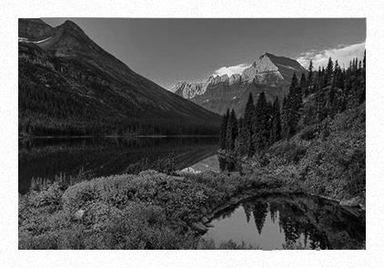
Figure 2: Our flattened query image
Downsample: Next we resize our image down to a thumbnail size. By doing this, we further simplify the later stages of the pipeline without losing too much of the structural information of the image, and we also gain some measure of scale invariance.
The thumbnail is of symmetric size, and its width is dictated by the uiThumbSize parameter. The larger the thumbnail, the greater our precision, so the entire hash function is scalable by this variable hash size parameter.
One final consideration for our downsample operation is the method by which we reduce the resolution. Insight uses a coverage filter in order to quickly perform large downsample operations without suffering from sampling error. Alternatively, we could use an iterative method such as generating a bilinear mip chain and selecting the lowest resolution level.
Transform: Next we transform our thumbnail image into frequency space using the discrete cosine transform. This decorrelates our pixel data into its frequency coefficient set and allows us to separate structural information (the low frequencies) from detail information (the high frequencies).
We then discard all values except for the upper left 1/16th of the image.
Average: Next we compute the average value of the AC coefficients in our 1/16th image. We do this simply by summing all values of our image, except the first, and dividing the result by the size of the image. We ignore the first (or DC) coefficient during this calculation because it would most likely distort our average.
Create our hash: Our final step is to generate our hash value. Our hash has a size of uiHashSizeInBytes, which means that we have reserved a certan number of bits for each pixel in our 1/16th image.
The bitrate per pixel will equal:
    UINT32 uiHashBitsPerPixel = ( uiHashSizeInBytes << 3 ) /
                                ( uiThumbSize * uiThumbSize );
We now traverse our image and for each pixel we subtract the average value (computed in the previous step), and then quantize the results. The degree of our quantization is based on the hash per pixel bitrate, with higher bitrates resulting in less quantization and thus lower error. Once we've quantized a value, we write it to the output stream that defines our hash.
This step measures the relative characteristics of the transform coefficients, rather than the values themselves, which allows us to compare images with different contrasts or other color adjustments.
CompareImages Implementation
Now that we've defined our hash method, we can return to CompareImages and give it a proper description.
If we simply computed the hashes of two images using HashImage, we could directly compare the values to determine if the images are identical. But this isn't exactly what we're interested in, since we want to perform a fuzzy comparison to determine the similarity of the images. To accomplish this, we compute the Hamming distance between the two hash values. The result will tell us how many bits are different between the two hashes, which we can then easily translate into a percentage.
We're almost finished, but there is one remaining issue. Let's say we compare our query image against a candidate that happens to simply be a rotated version of the query image. Our HashImage function will inform us that the two images are significantly different because they exhibit very different structure. Depending upon the application, this may or may not be a problem.
Fortunately, CompareImages was designed to be rotationally invariant, and is able to accurately compare images despite any rotation. It does this by incrementally rotating one of the two images from 0-360 degrees, and repeatedly comparing the hash value against that of the other image. We keep track of the best match, and return this value as a percentage.
As a further extension, CompareImages can also be instructed to test for flipped or mirrored images in the horizontal and vertical planes.
Results
Returning to our query image we can compare it against modified versions of itself in order to test the robustness of our perceptual hash comparison. In this first case, we've crystalized the query image and distorted it in a manner that maintains the overall structure.
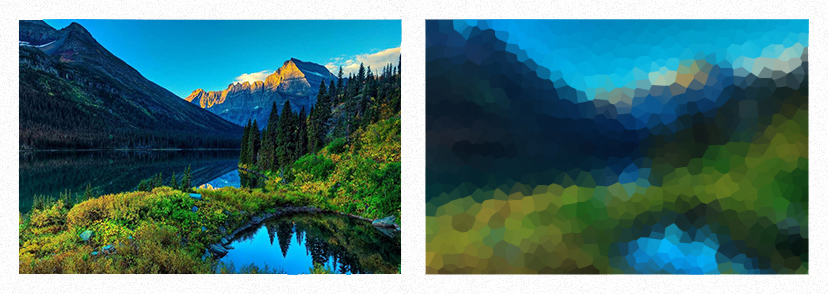
Figure 3: (Left) The original unmodified query image. (Right) A distorted version of the query image created using the crystalize filter in Photoshop.
Comparing the two images in Figure 3 with Insight yields a 98% similarity rating. Although we've distorted the second image, it still retains its basic structure and values. The thumbnail versions of both images are very similar, so a high similarity is not unexpected.
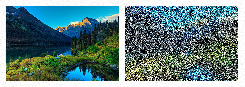
Figure 4: (Left) The original unmodified query image. (Right) A distorted version of the query image created by increasing the contrast and adding significant high frequency noise.
Comparing the two images in Figure 4 with Insight yields a 95% similarity rating. We've distorted our second image by introducing significant noise as well as increasing the contrast.
The high frequency noise almost entirely affects the higher frequency coefficients (which we discard), and our contrast change increases the magnitude of the coefficients from the average, but not their sign. Thus, neither of these modifications significantly changes our structure, so our similarity rating remains high.
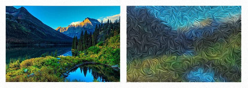
Figure 5: (Left) The original unmodified query image. (Right) A distorted version of the query image created by adding a visual swirl over the image.
Comparing the two images in Figure 5 with Insight yields a 96% similarity rating. We've distorted our second image by introducing a swirl artifact. Similar to previous results, this affects the higher frequency values more than the low, but the general structure remains intact.
So far we've analyzed images that are obviously quite similar, so these high similarity ratings are not unexpected. As user "Jemaclus" correctly points out on this Hacker News thread, another important test of a perceptual hashing system is whether it can properly detect dissimilarity between images.
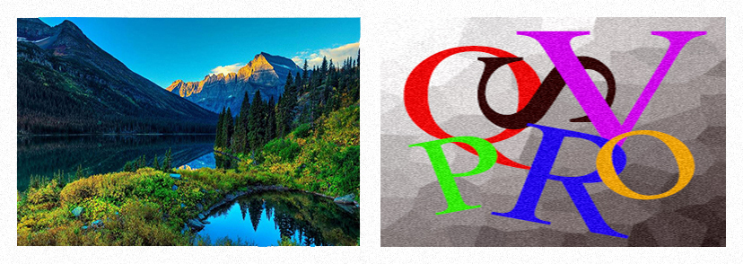
Figure 6: (Left) The original unmodified query image. (Right) A simple generated image that is deliberately different from our query image.
Comparing the two images in Figure 6 yields a similarity rating of 32%. This value is unsurprisingly high because of the way that we compute the hash. By decimating the information content and then measuring the Hamming distance between the two images, we have significantly increased the chances of a falsely high confidence (versus a direct image comparison).
To account for this, we consider ratings of 90% and above to signify high similarity, while ratings between 70-90% are possible similarity and values below 70% indicate dissimilarity.
Conclusion
Perceptual image hashes provide a useful way of quickly comparing the similarity of two images. This technique will not detect similarilty across large structural changes, but it does prove useful for certain applications like reverse image searches and other approximate comparisons where you can compute the hashes of images in a database as an offline process.
Note that when using Insight to perform comparisons, it is important to select an appropriate hash size that balances performance and accuracy. I used 64 bit hashes for the tests in this post, but I usually rely upon 128 bit hashes for larger scale comparisons.
More Information
For more information about Insight including source code, check out its project page. Also, be sure to check out pHash, a sophisticated perceptual image and audio hashing engine.
